Intro
Drug-resistant epilepsy affects millions worldwide, and one of the only ways to heal patients is neurosurgical resection of the epileptogenic zone. Detecting the seizure onset zone, which is one of the main indicators of the epileptogenic zone - together with potential physical lesions seen through an MRI scan - is a time consuming process for many neuroclinicians and is subject to inter-observer variability. Helping them pinpoint the SOZ automatically from SEEG signals - which they are trained to look at manually - would not only save them time but - if the models are accurate enough - could be better than a human annotator, potentially improving brain surgery outcomes. Our efforts go into that direction. There are other less invasive imaging techniques that are used to pinpoint the SOZ (MRIs, PET, CT scans and MEG), but the most invasive of them all, SEEG, remains the gold standard.
Problem definition
We are given multi-variate stereo-EEG time series, with a variable number of channels, duration, and outside and during seizure events. We want to predict for each channel of that time series, the likelihood that is part of the SOZ. We aim to develop a method that reliably generalizes to unseen patients, and that can train across a diverse set of patients from different centers.
Two-stage transformer encoder - SOZFormer
We developed and trained a two-stage transformer encoder for SOZ detection. The first, temporal stage uncovers relationships between 5 second clips in a sequence of size S=25 through multi-head attention.
The spatial encoder then finds the relationships between the different channels, and a final classification head allows us to compute channel-wise SOZ probabilities by averaging performance across training sequences. This approach puts our faith in a deep learning model to find the seizure onset zone directly, without relying on human-learned heuristics (like pre-computing very special features such as spikes and HFOs).
This is in line with the ideas of Richard Sutton and the Bitter Lesson, an essay that explains that techniques that leverage computing end up winning when scaling data and compute, compared to basing our models on heuristics. We believe this is the right path for research in this area: even though expert neurologists debate different things to look for in the signal, a well crafted DL model can find complex SOZ-indicating patterns in the signal that are hard for humans to detect and investigate.

This model was trained using 2 H200 GPUs on the coc-gpu cluster. It is divided up in a few logical blocks:
- Tokenizer: creates the tokens for the temporal stage using a Db-2 Wavelet Packet Transform with 5 levels of decomposition (2^5 frequency bins) for time-frequency features + an MLP to reduce input feature size.
- Temporal encoder: transformer encoder using multi-head self attention on the time tokens for each given channel
- Temporal encodings summarizer: Summarizes the temporal output sequence for each channel into one representation (Concatenation + MLP)
- Gather the summarized channel embeddings as an input sequence to the spatial encoder
- Individually apply an MLP classification head to each output channel representation to obtain output logits (non-normalized)
- Apply a sigmoid to obtain SOZ scores.
A word on implementation
Implementation done in Pytorch, trained on two GPUs using DataParallel. Detailed code can be found on our Github.
Data Distribution
For the final training run, we decided to use a private dataset from a French hospital (CHUL) with patients with large recording durations, in addition to HUP and EIIMD. Most of the clip sequences will come from CHUL, so we should expect better performance on that dataset. An upcoming parternship with the GT SIPLab and Emory's neurology department wil give us access to many more patients, enabling us to improve generalization performance of this model.
EIIMD and HUP contain many more ictal (meaning seizure events) recordings than interictal recordings, unlike CHUL which contains many long interictal recordings. In order to make our model as general as possible, we use both, with patients from different centers. Also note that this SOZ detection problem suffers from an ~80% inter-labeler agreement rate (meaning different neurologists labeling the SOZ would agree on ~80% of SOZ-labeled channels)

A special loss function
Our channel classification problem is heavily unbalanced, and only ~10% of stereotactic contacts in a given patient are part of the SOZ. To address that, we employ a focal and class-balanced binary cross-entropy loss. This loss function down-weights the contribution of easy examples and focuses training on hard negatives. The formulation is given by:
$$ L_{\text{FCBBCE}} = -\frac{1}{| I |} \sum_{i \in I} {w_i}^{CB} (1-{p_t}^i)^\gamma \log({p_t}^i) $$$$ w_i^{CB} = \frac{1 - \beta}{1 - \beta^{N_{y_i}}} \quad \text{$\beta \in [0,1[$ tunable hyperparameter, $N_{y_i}$ number of examples in the batch with same label as $i$} $$
Here, $w_i^{CB}$ represents the class-balancing weight, and $\gamma$ is the focusing parameter. The term ${p_t}^i$ reflects the model's estimated probability for the true class, defined conditionally based on the ground truth label $y_i$:
$$ {p_t}^i = p_i \mathbb{1}[y_i = 1] + (1-p_i) \mathbb{1}[y_i=0] $$In this context, $\mathbb{1}[\cdot]$ denotes the indicator function, which evaluates to 1 if the condition is met and 0 otherwise.
For this training run, we slightly simplified the loss by not using the focal power ($\gamma=0$), and we set a reasonable class balancing with $\beta=0.999$.
Training card
This summarizes the data parameters (batch size, temporal sequence length, individual clip duration, number of CV folds), model parameters (number of layers and hidden dimension sizes, dropout, number of attention heads), as well as the patient IDs included in each cross-validation fold, for the sake of reproducibility. Feel free to zoom in to see detailed information.
The test folds taken together constitute a partition of patients, and for each fold the remaining patients are split randomly between train and validation (15% val, 85% train among the remaining 80%).

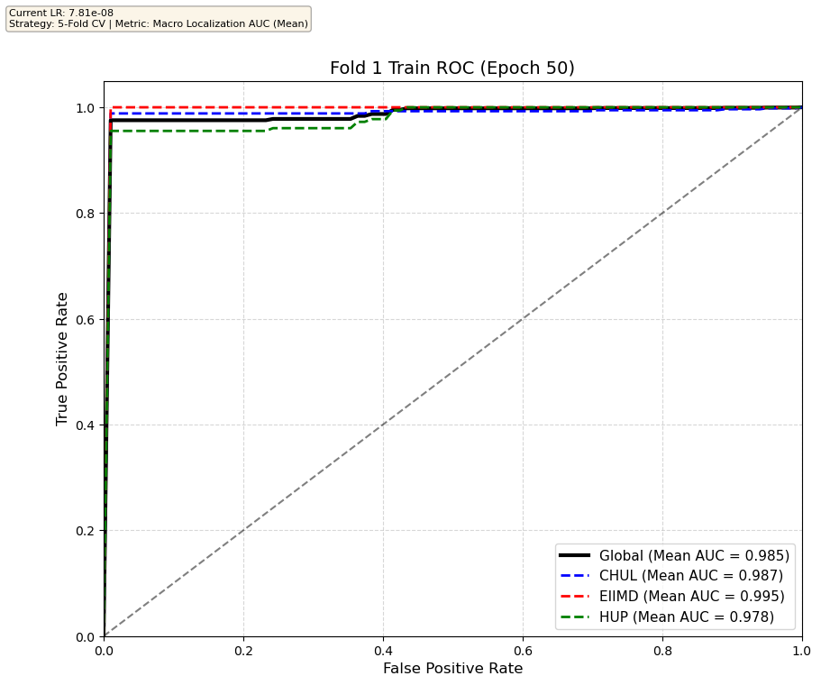
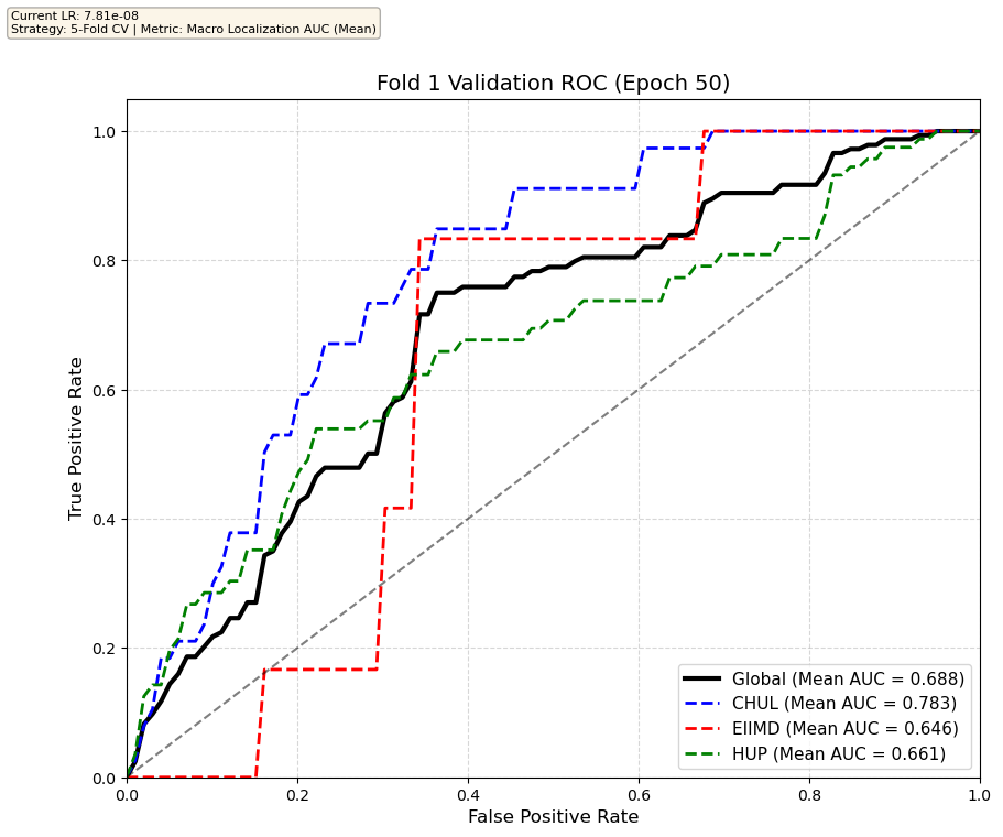
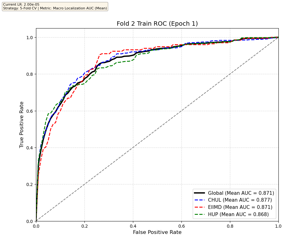
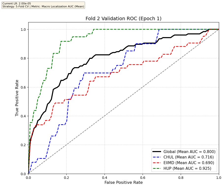
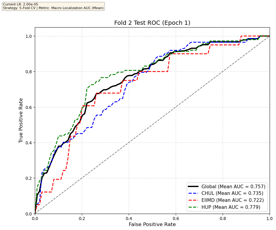
Transformer training results on one of the five folds
We compare performance on the different datasets Receiver Operating Curves through training. We do 5-fold patient-wise cross-validation.
Unfortunately, when we decided to implement CV, our training run stopped at ~7.5 hours and finished training for the first fold and barely started the second fold, so we only present training for the first fold and the start of the second fold. With more training time, we'd be able to get a full cross-validation performance. At least the code is implemented, but a more significant amount of time is necessary to do full 5-fold CV. This is one of the difficulties with using larger deep learning models like transformers.
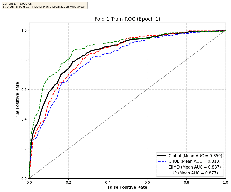
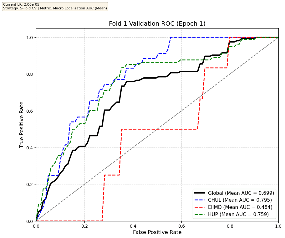
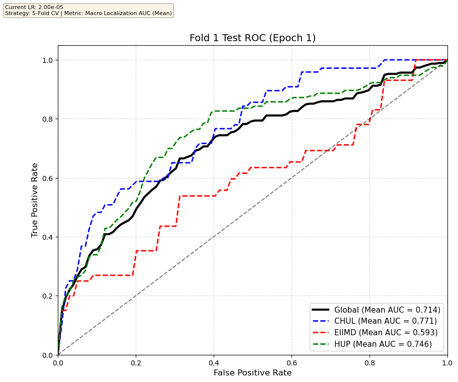
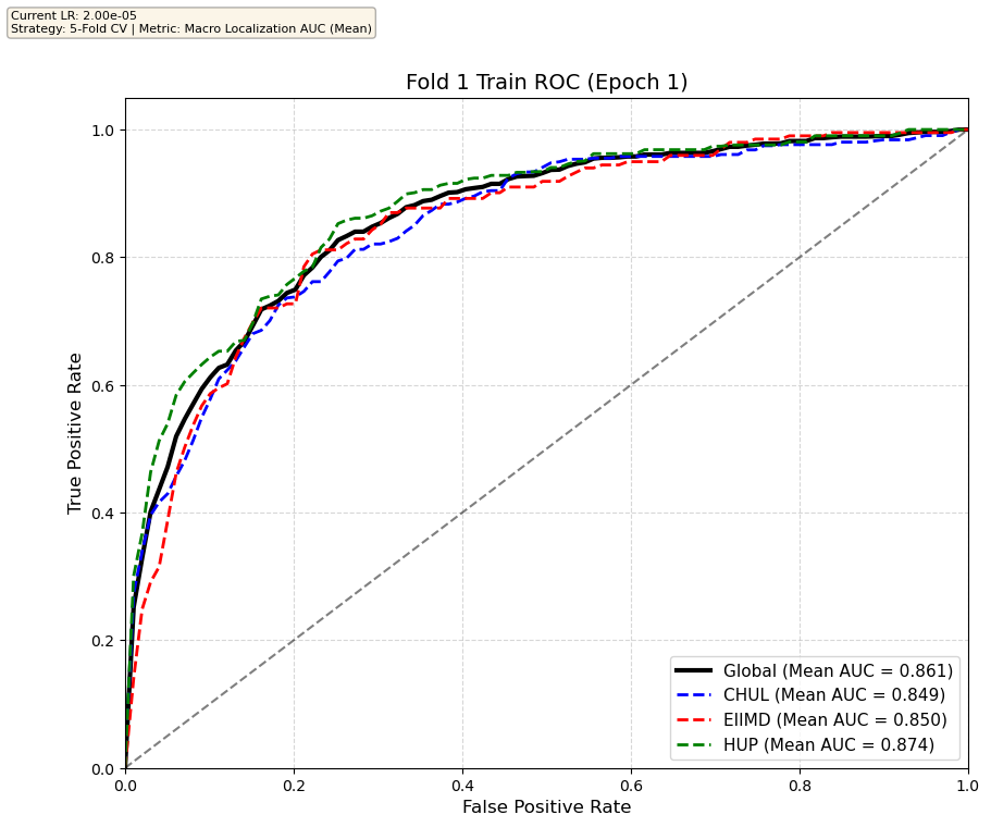
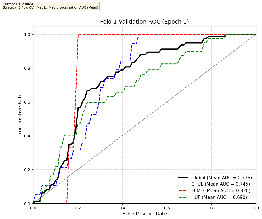
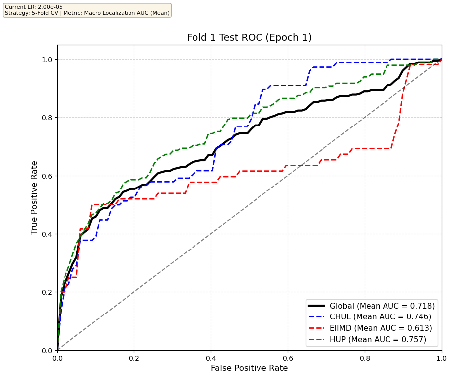
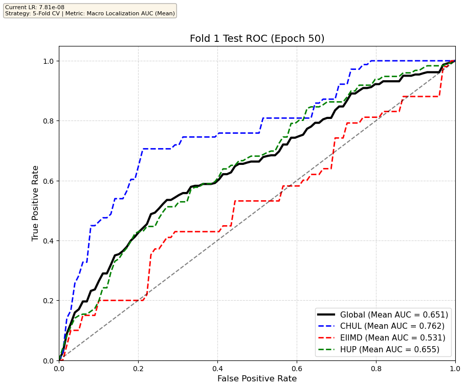
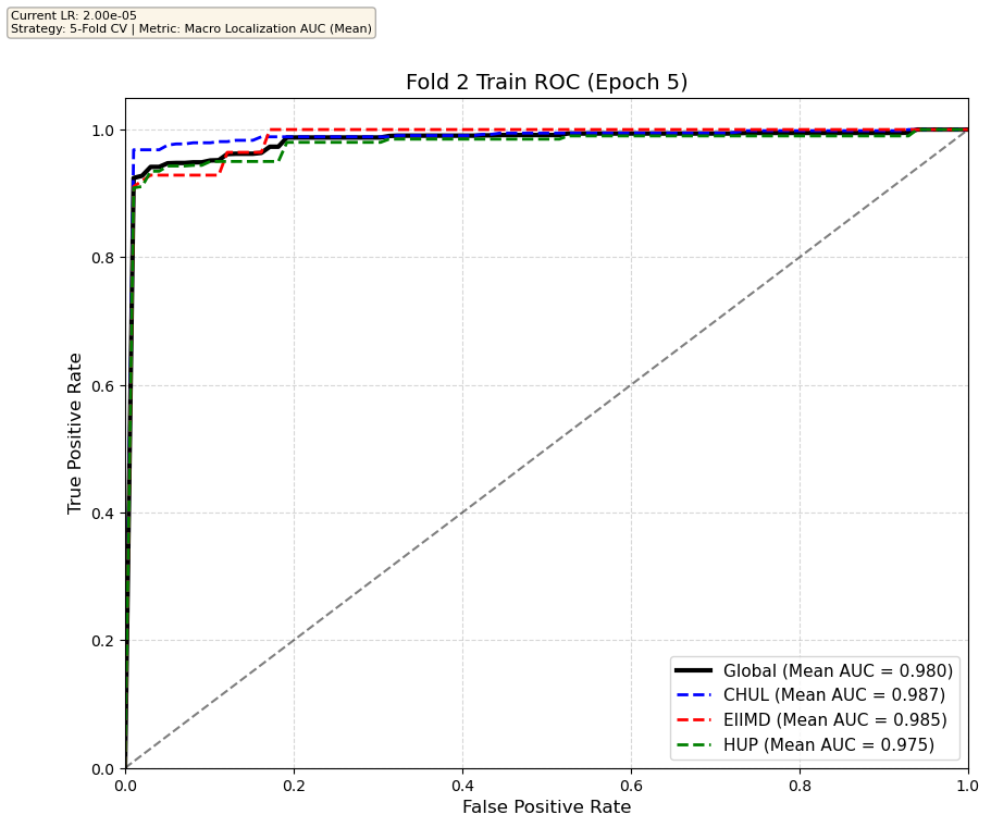
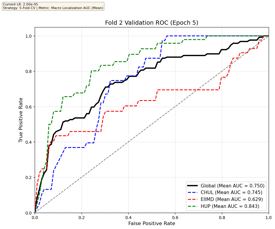
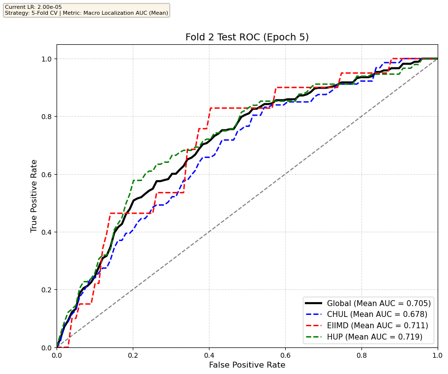
Performance increases in order of data availability for the different datasets. EIIMD recordings are just 10 or 20 minutes long, we have recordings that are a bit longer for a lot HUP patients (up to 40 minutes), but CHUL has recordings that can last up to 20 hours.
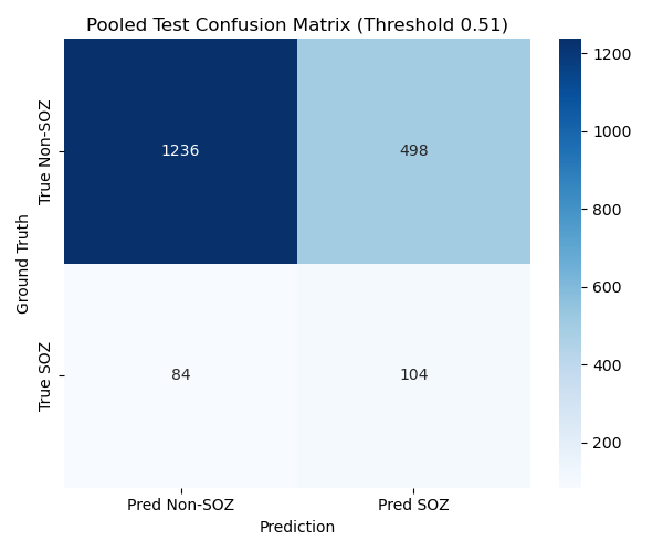
Test set confusion matrices for the two first folds
We find the threshold that maximizes the J-statistic on the validation set, and look at test set performance. We report channel-wise confusion matrices on the test set for fold 0 and 1, as well as patient-wise classification metrics (we compute these metrics for each patient channel-wise, then average across patients; this gives a more realistic estimate of model performance than just looking at the metrics channel-wise, because different patients have different number of implanted channels), with mean and standard deviation, for each fold.
First fold
| Metric | First fold Test Set Mean | First fold Test Set Std |
|---|---|---|
| Macro Recall | 0.5801 | 0.378 |
| Macro Specificity | 0.7243 | 0.0748 |
| Macro Precision | 0.1877 | 0.1572 |
| Macro F1 Score | 0.2931 | 0.1716 |
Second fold
| Metric | Second fold Test Set Mean | Second fold Test Set Std |
|---|---|---|
| Macro Recall | 0.5957 | 0.2783 |
| Macro Specificity | 0.6883 | 0.2945 |
| Macro Precision | 0.2468 | 0.1340 |
| Macro F1 Score | 0.3194 | 0.1261 |
Performances like these are arguably not good enough to be used clinically, as the model misses a little less than half of the SOZ channels, and there are still quite a lot of false positives. But the results are encouraging, and we can hope for a clinically useful model with more data, more hyperparameter tuning and longer training runs. We also observe a lot of inter-patient variability: some patients are way easier to classify than others. Also note that the validation sets that were used are not super significant (5 or 6 patients to validate), so more training data would definitely be a good thing. The approach is sound and deserves more exploration.
Conclusion on SOZFormer
The transformer based model has a great memorization capacity and quickly achieves perfect performance on the training set, and is still able to generalize quite well to unseen patients (~75% to 80% Global AUC on test and validation sets), although the model starts overfitTing and performance degrades after a few epochs. Very long training runs might be able to counter that overfitting, since transformers are prone to deep double descent. This is a good sign that scaling this model with more data and careful training would yield very good results.
SOZFormer TODO List
- Obtain Emory Neurology department data via SIPLab (>400 patients!)
- Longer and complete training runs
- Careful hyperparamter tuning
- Implement positional encodings for the temporal stage, as that would probably meaningfully impact training performance. Right now the model sees the S=25 tokenified clips as a disordered set, although they are ordered in time.
Diffusion Convolutional Recurrent Neural Network (DCGRU)
Model presentation
This model relies on graph diffusion on a fixed connectivity graph (either undirected or directed connectivity) between the different channels (unlike the variable attention mechanisms inside the transformer), inside a modified Gated Recurrent RNN unit. Chaining these units allows us to build a recurrent neural network, used in:
- A self-supervised pretraining task that consists in predicting the next sequence DFTs (Discrete Fourrier Transform)
- A finetuning task that we modified from the original paper to do SOZ detection instead of seizure event detection
Methodology: Spatiotemporal Modeling
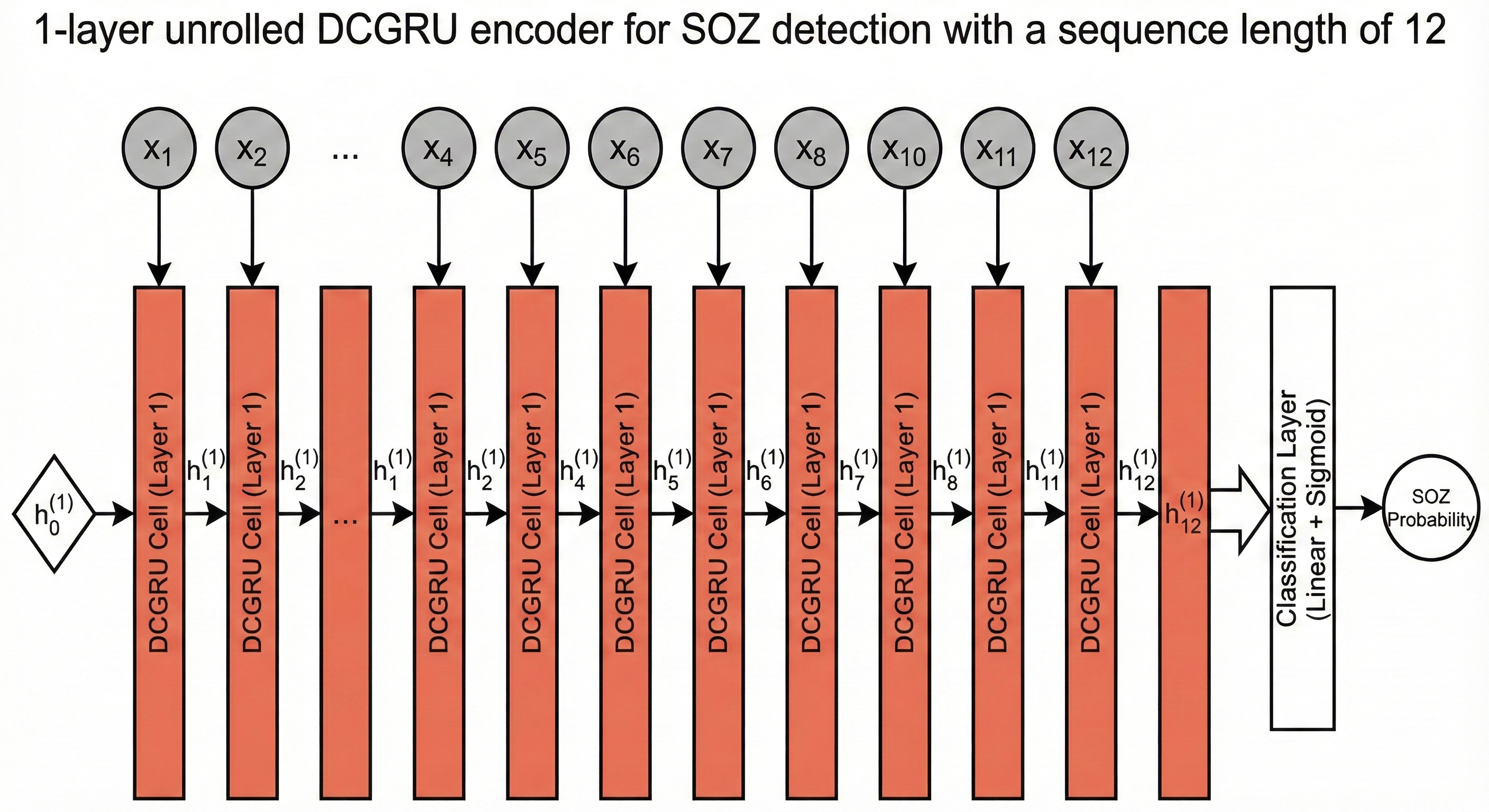
Seizures are complex events that evolve over both space and time. To capture this, we re-purposed a DCGRU - a hybrid model unifying Graph Diffusion and Gated Recurrent Units. Our architecture features a 1-layer encoder unrolled over 12 time steps. This allows us to track how a seizure propagates across brain regions.
FFT Preprocessing: Instead of raw signals, we preprocess our inputs using Fast Fourier Transform (FFT). This gives us 2,500 spectral bins per channel, explicitly exposing High Frequency Oscillations (HFOs) - a critical biomarker for seizure zones that standard models often miss.
Dynamic Graph Learning: Brain connectivity isn't static, so we don't use a fixed graph. Instead, we compute the Adjacency Matrix dynamically for every batch using Pearson Correlation. This allows the model to adapt to the patient's changing brain state during the recording.
Handling Class Imbalance: Seizure Onset Zones are rare—less than 10% of the data. We implemented a Weighted Loss function (BCEWithLogitsLoss with pos_weight) to heavily penalize missing a seizure. This forces the model to prioritize Recall.
Here is what the unrolling process looks like for 5 clips per sequence in a 3 layer DCRNN

Or for a simiplied implementation (ours) with just one layer
This is the original figure from the paper describing the model, for a simpler downstream task of seizure detection, instead of spatial seizure onset zone detection
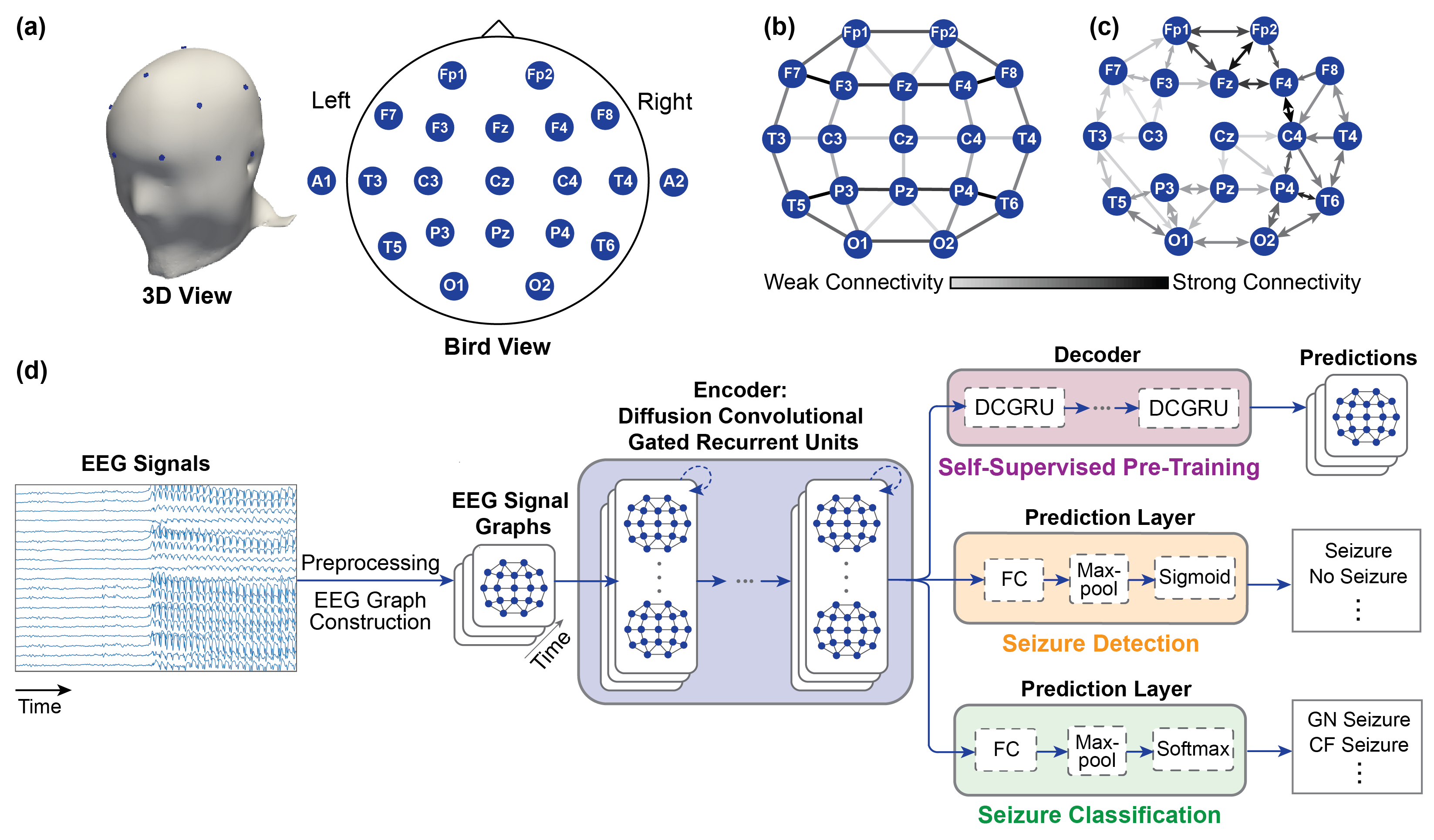
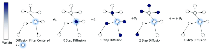
Illustration of the diffusion convolution process inside each DCGRU cell. Source
Data
Only HUP and EIIMD were used for that training run, and there was a single train/test/validation split across all patients, no CV (this is a TODO item, and must be done on the same sets as SOZFormer to provide a completely fair comparison, but this is work left for a future publication).
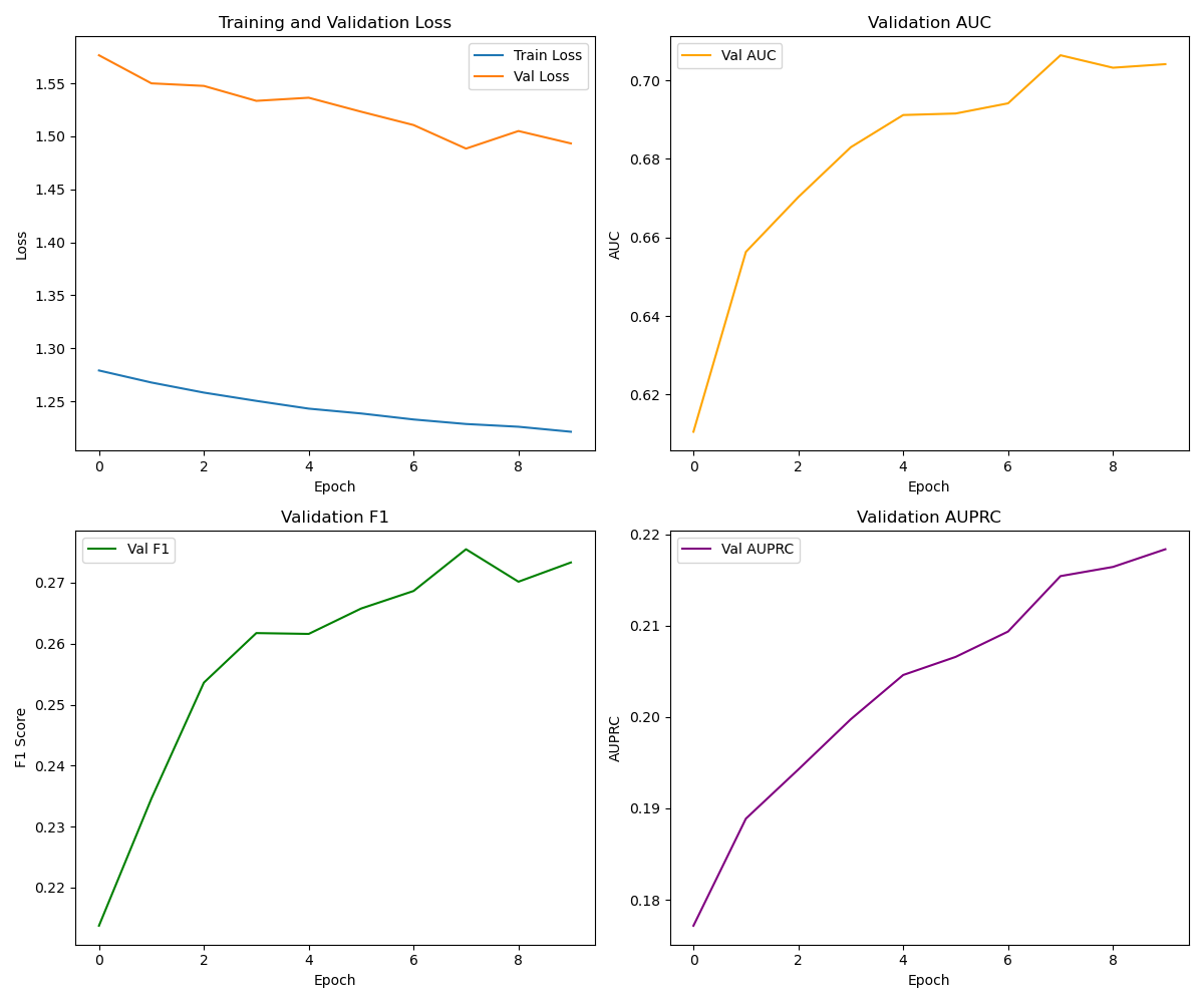
Training dynamics
The training curves confirm our strategy worked. We observe steady convergence in the Loss (top left). Note that while the Training and Validation loss lines do not touch, they both trend downwards, indicating the model is learning robust features without overfitting. The gap is expected due to the cross-patient split difficulty.
More importantly, the rising AUPRC (Area Under Precision-Recall Curve) (bottom right) proves the model is successfully identifying those rare positive events without being overwhelmed by false alarms. The F1 score also trends upwards, showing a better balance between Precision and Recall.
Results
Learning Evolution: Training spatiotemporal graphs from scratch is difficult. We used Transfer Learning, initializing our encoder with weights from a self-supervised task (next-step prediction). This gave the model a massive head start.
Epoch 1 The model starts with a decent baseline but struggles to separate classes.
Best Epoch Performance peaks at an AUC of ~0.70. The curve bows strongly to the top-left, indicating robust separation between SOZ and non-SOZ channels.
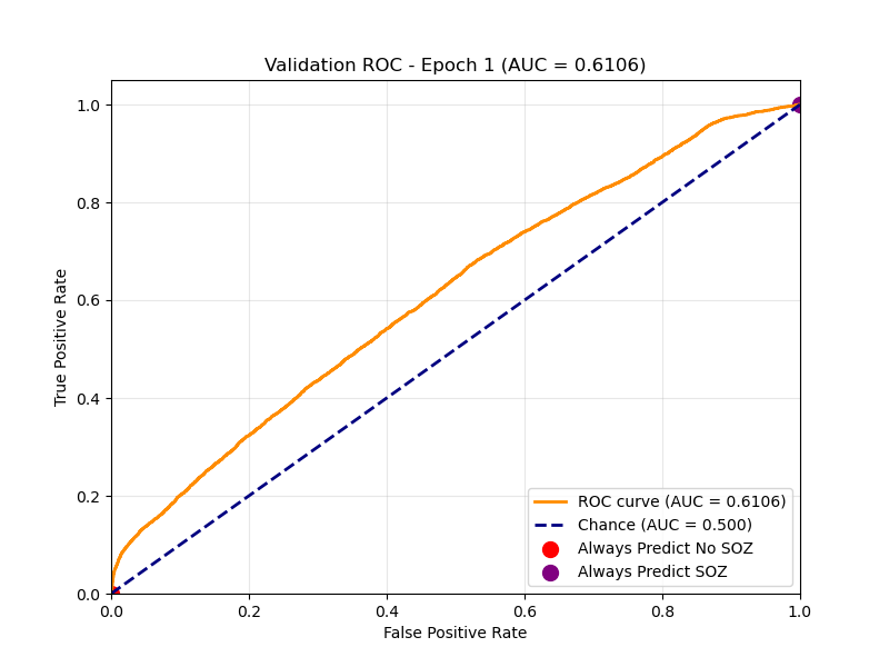
Epoch 1 ROC
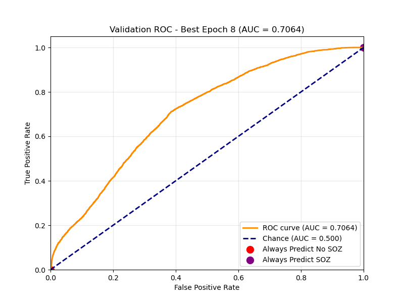
Best Epoch ROC
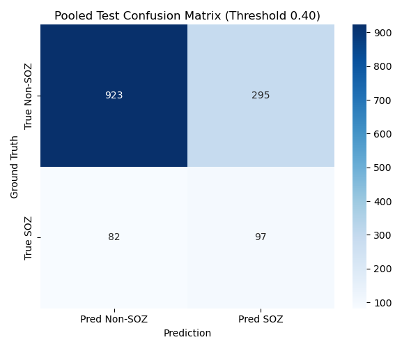
Final Test Set Performance:
On the held-out Test Set (unseen patients), we achieved an AUC of 0.64 and a Recall of roughly 55%. In a clinical setting, Recall is paramount as we cannot afford to miss a potential onset zone.
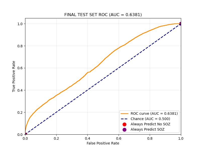
| Metric | Test set Mean |
|---|---|
| AUC (Channel-wise) | 0.6381 |
| Recall | 0.5487 |
DCGRU TODO List
- Implement 5-Fold Cross-Validation for fair comparison with SOZFormer.
- Integrate SIPLab Data (>400 patients) to improve generalization.
- Hyperparameter Tuning (optimize
num_rnn_layers,seq_len,hidden_dim). - Longer Training Runs to investigate convergence behavior.
- Use the same CV logic and metrics as for the SOZFormer (5-fold CV) and use patient-averaged performance instead of channel-wise metrics
SVM Model
For this model, we focused on using per-channel heuristic signs of the SOZ and then used an SVM to classify each channel independently, without relying on the potential connectivity network that exists between channels, unlike the two previous methods.
Features
- HFO/Spike features - "events"
- Wavelet features
We use an algorithmic spike detector that doesn't rely on a machine learning model, then used the per-channel spike counts as a feature for training, as well as WPT based per-channel features.
Model
We use an SVM with an RBF kernel with balanced class weighing.Results
On the right: channel-wise confusion matrix for the test set with a default threshold of 0.5. On the left: channel-wise confusion matrix for the test set with an optimal threshold that maximizes Youden's J statistic on the test set (this should be on the validation set, we souldn't be able to use test labels, but it still gives us an idea about optimal threshold selection - obviously we cannot do this on unseen data).
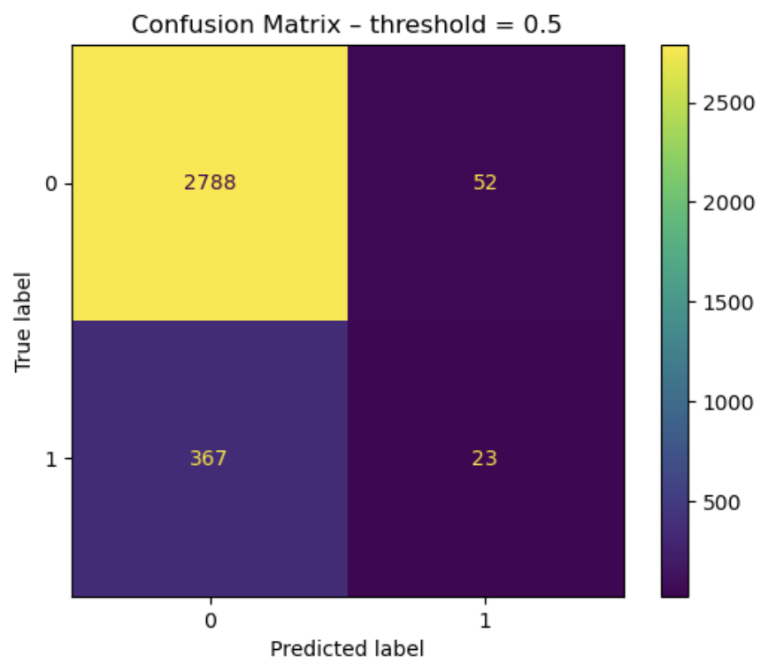
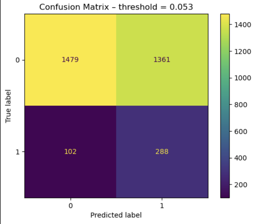
| Metric | Test Set Mean (with optimal threshold on test set - TODO on validation) |
|---|---|
| Precision | 0.17 |
| Recall | 0.74 |
| F1 Score | 0.28 |
Project Conclusion & Future Outlook
We are extremely proud of the progress achieved during this course. We have successfully established strong baselines with our SVM and DCGRU models and laid the groundwork for a robust benchmarking pipeline for Seizure Onset Zone detection. We remain confident in the high-impact publication potential of our work, particularly the SOZFormer architecture. We are committed to continuing this research, refining our models, and rigorously validating our results until the work is publication-ready. Several team members plan to carry this momentum forward, with the specific goal of submitting our findings to NeurIPS.
References
-
Tang, S., Dunnmon, J., Saab, K. K., Zhang, X., Huang, Q., Dubost, F., Rubin, D., & Lee-Messer, C. (2022).
Self-Supervised Graph Neural Networks for Improved Electroencephalographic Seizure Analysis.
International Conference on Learning Representations (ICLR).
Available at: https://openreview.net/forum?id=k9bx1EfHI_- -
Vaswani, A., Shazeer, N., Parmar, N., Uszkoreit, J., Jones, L., Gomez, A. N., Kaiser, Ł., & Polosukhin, I. (2017).
Attention is All you Need.
Advances in Neural Information Processing Systems (NIPS).
Available at: https://proceedings.neurips.cc/paper/2017/hash/3f5ee243547dee91fbd053c1c4a845aa-Abstract.html -
Wang, Y., Yang, Y., Li, S., Su, Z., Guo, J., Wei, P., Huang, J., Kang, G., & Zhao, G. (2022).
Automatic Localization of Seizure Onset Zone Based on Multi-Epileptogenic Biomarkers Analysis of Single-Contact from Interictal SEEG.
Bioengineering.
Available at: https://www.mdpi.com/2306-5354/9/12/769 -
Gunnarsdottir, K. M., Li, A., Smith, R. J., Kang, J., Korzeniewska, A., Crone, N., et al. (2022).
Epilepsy-iEEG-Interictal-Multicenter-Dataset.
OpenNeuro.
Available at: https://nemar.org/dataexplorer/detail?dataset_id=ds003876 -
Bernabei, J. M., Li, A., Revell, A. Y., Smith, R. J., Gunnarsdottir, K. M., Ong, I. Z., Davis, K. A., Sinha, N., Sarma, S., & Litt, B. (2022).
HUP iEEG Epilepsy Dataset.
OpenNeuro.
Available at: https://nemar.org/dataexplorer/detail?dataset_id=ds004100 -
Lin, T.-Y., Goyal, P., Girshick, R., He, K., & Dollár, P. (2017).
Focal Loss for Dense Object Detection.
International Conference on Computer Vision (ICCV).
Available at: https://ai.meta.com/research/publications/focal-loss-for-dense-object-detection/ -
Cui, Y., Jia, M., Lin, T.-Y., Song, Y., & Belongie, S. (2019).
Class-Balanced Loss Based on Effective Number of Samples.
Proceedings of the IEEE/CVF Conference on Computer Vision and Pattern Recognition (CVPR).
Available at: https://openaccess.thecvf.com/content_CVPR_2019/html/Cui_Class-Balanced_Loss_Based_on_Effective_Number_of_Samples_CVPR_2019_paper.html
Contribution table
| Zacharie Rodiere | Developed the SOZFormer, Cross-Validation and plotting logic. Wrote most of the final report. |
| Agam Saraf | Implemented DCGRU for SOZ detection and contributed to final report. |
| Austin Tsang | Helped out with the transformer model early on (start implementation that had to be redone). No contributions to the final report. |
| Anna Alexiou | Worked on RBF SVM implementation. No contributions to the final report. |
| Tyler Warner | Worked on SVM features. No contributions to the final report. |