Literature Review
Epilepsy affects over 50 million people worldwide, and about 30% of patients suffer from drug-resistant epilepsy, for whom surgery is often the only curative option. The success of surgical intervention depends critically on the accurate identification of the epileptogenic zone (EZ), specifically the Seizure Onset Zone (SOZ), the region where seizures originate.
Stereo-electroencephalography (sEEG), which involves intracranial recordings from depth electrodes, has become a gold standard for delineating the SOZ due to its ability to capture high-resolution spatiotemporal activity.
Key Biomarkers for SOZ Detection
- High Frequency Oscillations (HFOs): 80–500 Hz signals considered reliable markers
- Interictal Spikes: Interictal epileptiform discharges remain standard clinical markers
- Phase-Amplitude Coupling (PAC): Captures cross-frequency interactions
- Connectivity: Functional connectivity adds valuable information for SOZ localization
Traditional approaches rely heavily on expert visual review, which is time-consuming, subjective, and prone to inter-rater variability. Machine learning methods including CNNs, RNNs, GNNs, and Transformers have shown promise in automating this process.
Dataset Description
We employ multi-center datasets to ensure variability in acquisition protocols, electrode configurations, and patient demographics, enabling assessment of cross-center generalization.
De-identified patient data (n=58) containing electrophysiologic data for interictal and ictal periods from the Hospital of the University of Pennsylvania.
View DatasetDe-identified patient data (n=39) with sleep/wake annotations from multiple centers including NIH, Johns Hopkins, and University of Miami.
View DatasetProblem Definition and Motivation
For patients with drug-resistant focal epilepsy, surgical resection of the SOZ can be curative. However, the main clinical challenge lies in accurately identifying the SOZ from sEEG recordings. Mislocalization leads to failed surgeries and persistent seizures.
Current manual approaches are inefficient and limited by subjective interpretation. Our motivation is to develop machine learning models that can automatically detect the SOZ with high accuracy, robustness across datasets, and interpretability aligned with known biomarkers.
The project's impact extends beyond accuracy: automating SOZ detection can reduce diagnostic time, improve consistency, and potentially expand surgical candidacy by making evaluation more scalable.
Methods
This section outlines the preprocessing of sEEG signals and the model design for automatic SOZ detection.
Preprocessing
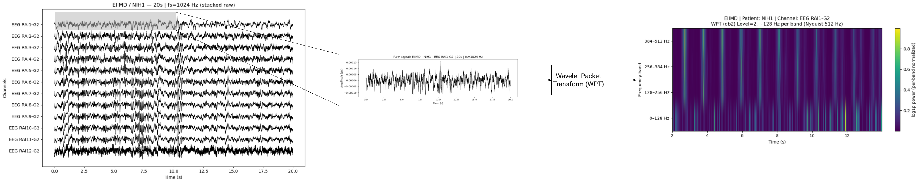
The sEEG signals at each electrode are processed by a Daubechies-2 (Db2) Wavelet Packet Transform (WPT). We use five levels of decomposition and this provides localized time–frequency features, useful for detecting spikes, ripples, and HFOs. The compact support of the Db2 wavelet allows sharp temporal resolution for transient spikes (i.e., sudden high-amplitude discharges), while its regularity suppresses smoother background activity. This granularity disentangles overlapping spectral components, allowing downstream models to identify ripples as sustained energy in specific sub-bands, and spikes as transient bursts in adjacent bands.
Implementation
A single-level Db2 DWT is implemented with torch.nn.functional.conv1d using analytical Db2
low-/high-pass filters. A recursive _wpt_recursive function performs full packet decomposition
on both branches up to level L = 5, yielding 2^L leaf sub-bands per channel.
Leaf outputs are concatenated to form the final WPT feature map.
Construct Db2 low/high filters from closed-form coefficients.
Convolve and downsample by two to obtain approximation and detail coefficients.
Apply packet decomposition on both branches at each level (L = 5).
Concatenate all 2^5 leaves into a compact per-channel WPT representation.
Model: Transformer-Based SOZ Detection with Contrastive Pre-Training
Design
We use a Transformer encoder that treats sEEG channels as an unordered set, enabling generalization across patients with varying channel counts and layouts. The model classifies each channel within a 10 s window from a sequence of 10 clips as SOZ vs. non-SOZ.
The model architecture consists of 5 main blocks:
tokenizer: passes each sample through WPT and an MLP to produce "tokens"
temporal encoder: takes the temporal tokens
for each channel and passes them through a transformer encoder layer
spatial preencoder: concatenates the temporal encodings and passes them through an MLP for a
lower_dimensional embedding for each channel
spatial encoder: passes the channel embeddings through a transformer encoder layer
projection head: passes the spatial encodings through an MLP to get the output logits
The Transformer architecture takes a 4d input with the following dimensions: Batch Size*Sequence Length*Num Channels*Num_Clips. Since the number of channels varies, we assume a max channel size and implement padding to ensure dimensions are consistent. So that the model knows what data is real and what is padding, a padding mask is generated and passed to the model along with the data. The padding mask is passed to each block so that they only perform computations for real data. The recording is also variable. However, instead of padding, we split the recordings into equal length sequences of 10 clips that are 10 seconds each. Any data that remains is discarded.
Input Tokenization
- For each sample, compute a Db2 WPT and pass the WPT features through an MLP.
- Positial encodings will be added in the future to help the model learn temporal relationships.
Training Strategy
Remove the projection head; add a linear + sigmoid classifier and optimize with focal class-balanced BCE.
Outputs & Interpretation
- Per-channel SOZ probability for each 10-second window.
- Attention maps provide interpretable, sample-specific connectivity patterns.
Results and Evaluation
This section will report quantitative performance on held-out patients and cross-center generalization. Once results are available, populate the summary cards and tables below. Suggested protocol and placeholders are provided for consistency and reproducibility.
Evaluation Protocol
- Unit of analysis: Channel-wise binary classification (SOZ vs. non-SOZ).
- Windows: 35 s non-overlapping (or specify overlap if used).
- Splits: Patient-level splits to prevent leakage; report cross-dataset transfer (train on one, test on another).
- Metrics: AUROC, AUPRC, Recall (SOZ), Precision (SOZ), F1 (SOZ), and Calibration (Brier score or ECE).
- Uncertainty: 95% CIs via patient-level bootstrap.
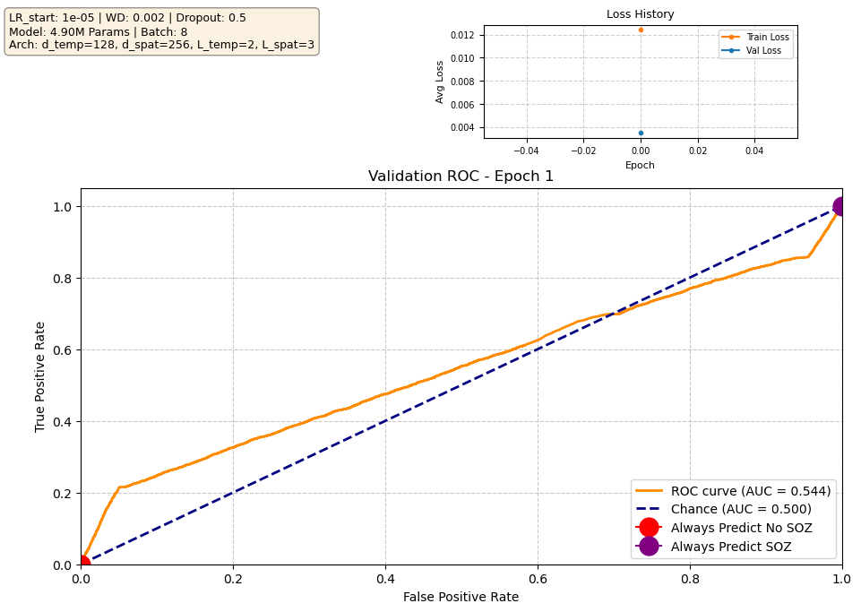
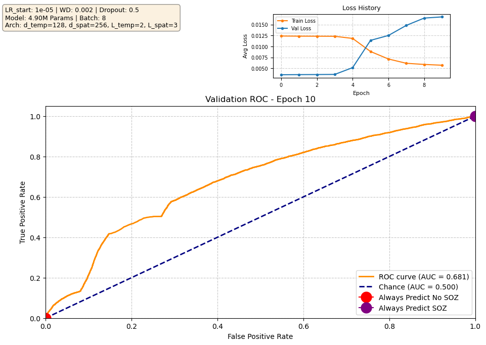
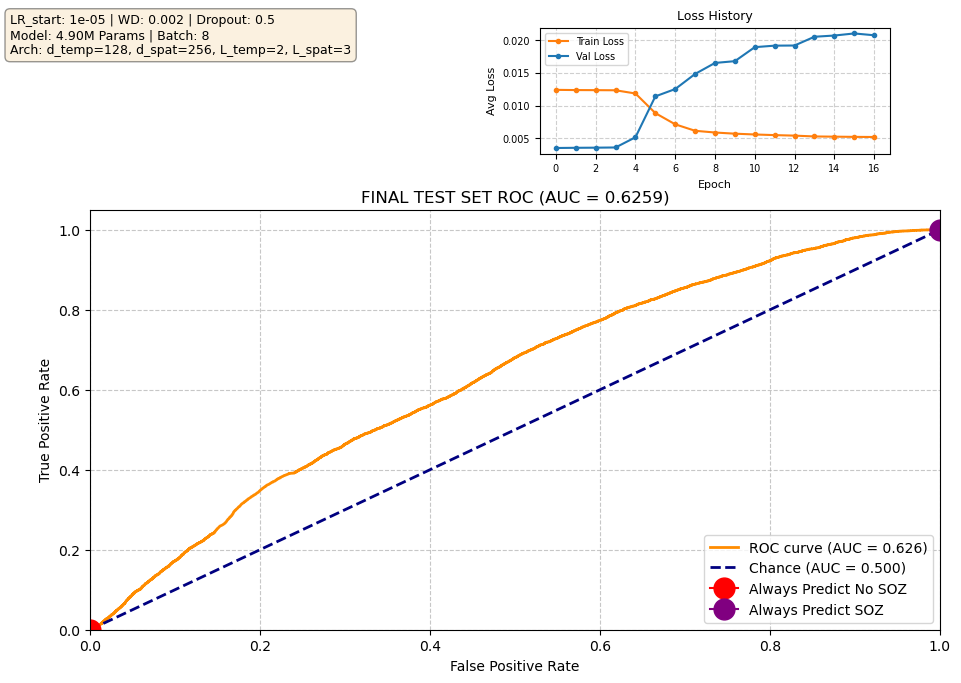
Our current best-performing model achieves a validation AUROC of approximately 0.70 at epoch 10. When evaluated on the held-out test set using the checkpoint from this best epoch, performance is reduced to ~0.63 AUROC, which indicates moderate generalization. Notably, the validation loss begins to increase after the early training epochs, while the validation ROC continues to improve. This is expected behavior: the loss penalizes the model for being confidently wrong, whereas the ROC measures only how well the model separates SOZ vs. non-SOZ channels. As training progresses, the model becomes more confident in its predictions, which increases loss when errors occur, even though the underlying class separation improves. In other words, the model’s probability calibration overfits before its ability to rank SOZ vs. non-SOZ channels does. Since ROC directly reflects separation ability — the priority in our task — the improving validation ROC is the more meaningful indicator of progress.